openUC2 Goniometer – Tutorial

Measure sessile-drop contact angles with your openUC2 modular microscope running ImSwitch on a Raspberry Pi.

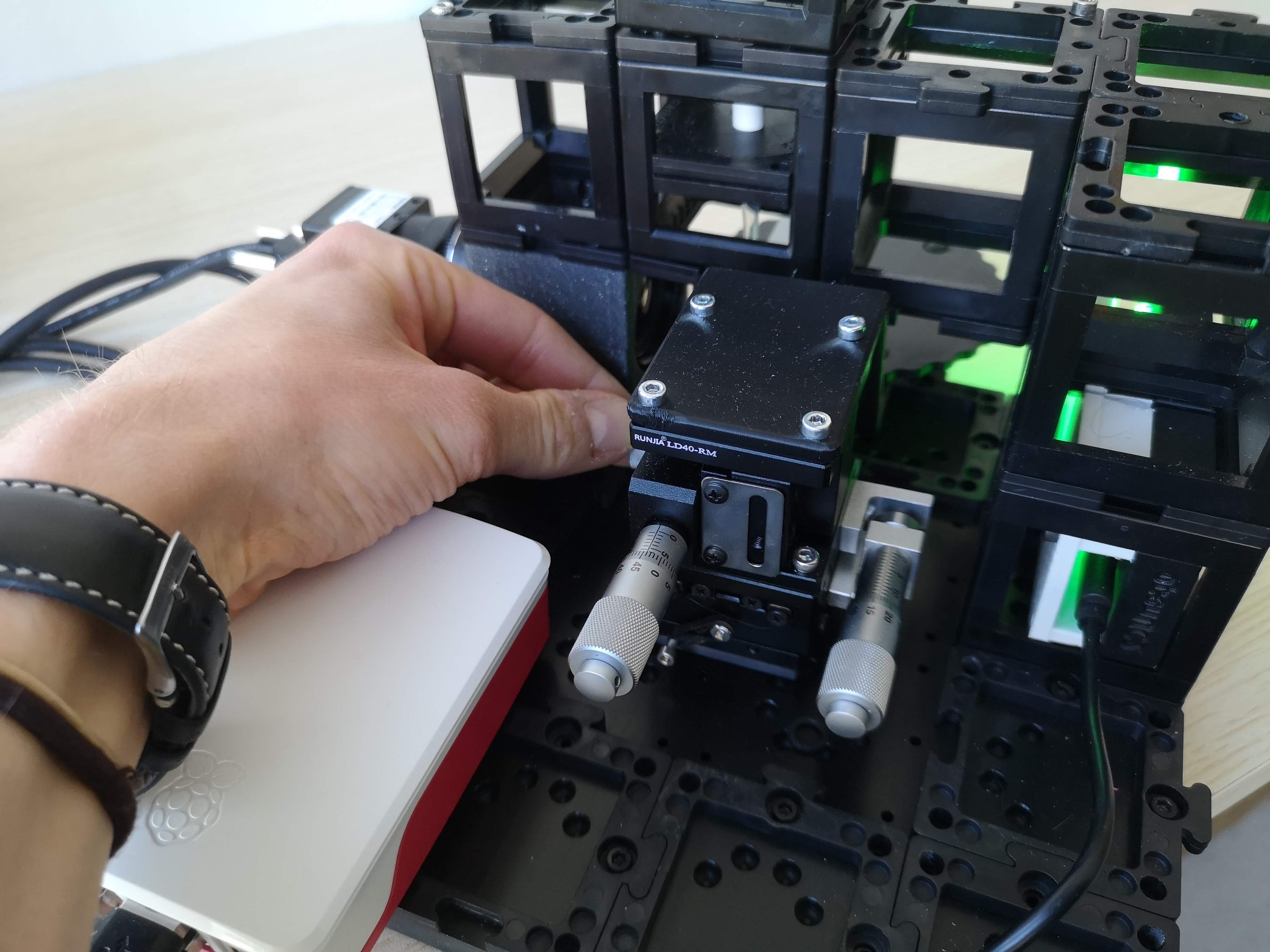
Beware: There are cubes inside :)

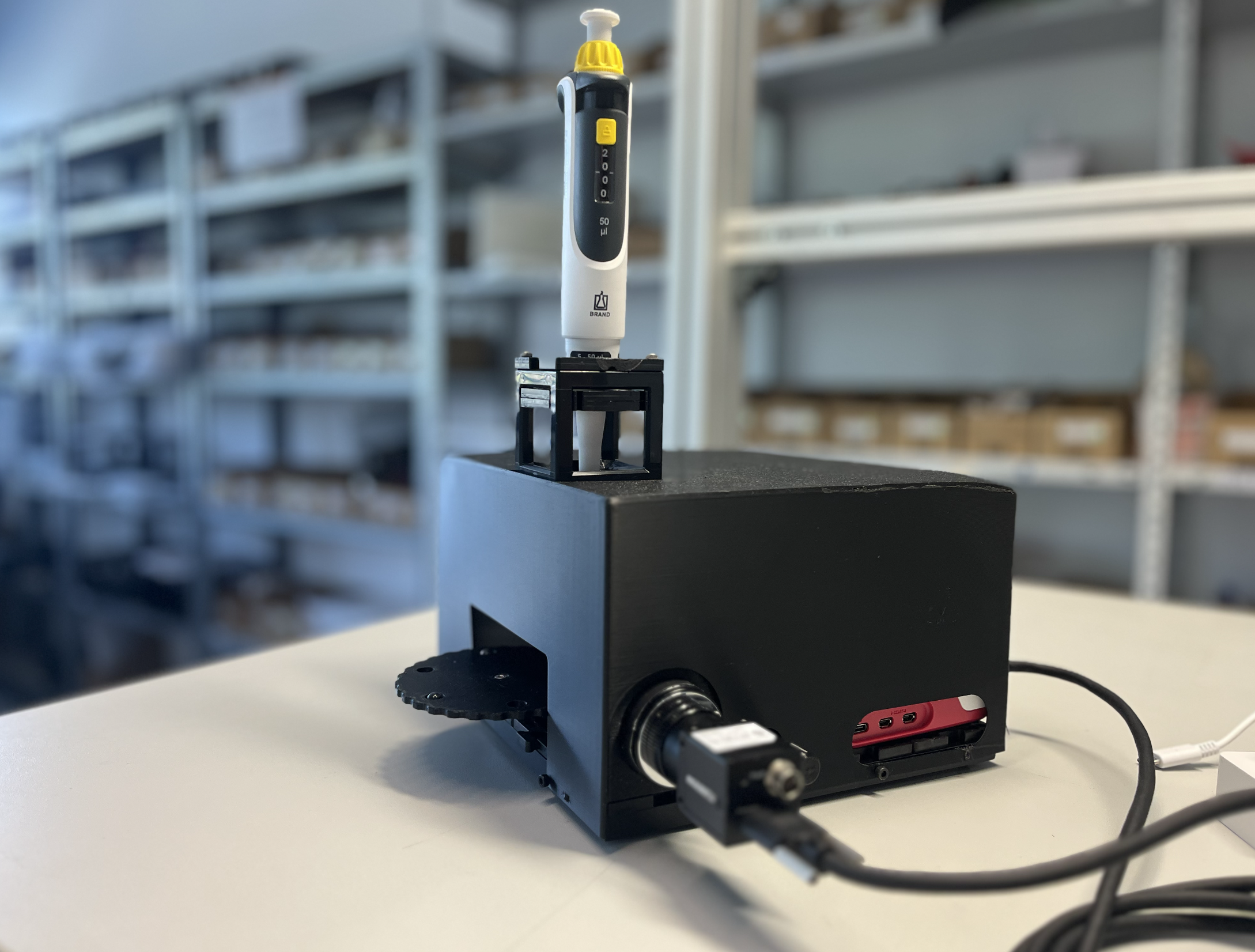
1. Hardware Overview

              ┌─────────────────────────────┐
              │      openUC2 Cube "Stack"   │
              │                             │
              │  ┌──────────┐               │
              │  │ Pipette  │  (syringe or  │
              │  │ Holder   │   dispenser)  │
              │  └────┬─────┘               │
              │       │ droplet             │
              │  ══════════════  substrate  │
              │                             │
              │  ┌───────────┐              │
              │  │HIK IMX178 │ USB3 camera  │
              │  │ CCTV Lens │  ~90° to drop│
              │  │    25 mm  │              │ 
              │  └───────────┘              │
              │                             │
              │  ┌──────────────────────┐   │
              │  │ LED Array + Diffuser │   │
              │  │  (back-light)        │   │
              │  └──────────────────────┘   │
              └─────────────────────────────┘
                        │ USB3
              ┌─────────▼──────────┐
              │   Raspberry Pi 5   │
              │   running ImSwitch │
              └────────────────────┘
                        │ Wi-Fi / Ethernet
              ┌─────────▼──────────┐
              │  Browser (laptop)  │
              │  ImSwitch UI       │
              └────────────────────┘

Component	Details
Platform	openUC2 modular cube system
Controller	Raspberry Pi 5 (runs ImSwitch)
Camera	HIK Vision IMX178 (USB 3.0, 6.4 MP, colour/mono)
Illumination	LED array + diffuser — back-lit, homogeneous
Dispensing	Syringe pipette held in a cube mount; drops ~1–10 µL
Substrate	Flat sample placed on the cube base plate

The camera observes the droplet from the side (macro view) so the contact line between the drop and substrate is visible as the widest horizontal extent of the drop silhouette.

2. Software Stack

Raspberry Pi
└── ImSwitch  (Python, FastAPI REST)
    └── GoniometerController  (plugin)
        ├── REST API  /GoniometerController/…
        └── OpenCV image processing pipeline

Browser
└── ImSwitch Frontend  (React)
    └── GoniometerController.js  (this UI)

ImSwitch exposes the goniometer as a REST API. The React frontend is served alongside ImSwitch and communicates over the local network.

3. In Action

The software workflow is explained in the following video. You have to connect to the Raspberry Pi's wifi or network (PW: youseetoo) and then navigate to the website http://192.168.4.1 and enable the Goniometer app in the side bar:

4. UI Walkthrough

The code for the backend is here: https://github.com/openUC2/ImSwitch/blob/master/imswitch/imcontrol/controller/controllers/GoniometerController.py

The code for the frontend is here: https://github.com/openUC2/ImSwitch/blob/master/frontend/src/components/GoniometerController.js

4.1 Live Camera Stream

The top-left card shows a live MJPEG stream from the HIK camera.

The stream is updated continuously — use it to position the pipette and focus the droplet before snapping.
Zoom and pan are available on the snapped image (bottom card), not on the live view.

4.2 Setting a Crop ROI

For best results the algorithm only sees the droplet and its reflection — crop out any background clutter.

Click the Crop icon (✂) in the live stream card header. The cursor changes to a crosshair and an info banner appears.
Click and drag a rectangle around the droplet (include a little background above and below).
Release the mouse — the crop is sent to the backend and a gold dashed rectangle persists on the live view.
To remove the crop, click the × on the orange "Crop active" chip, or click Reset Crop.

Why crop? The algorithm searches for the widest contour in the image. Bubbles, pipette edges, or substrate edges that extend further than the drop width will confuse the baseline detection.

4.3 Camera Settings

Below the live stream you find two fields:

Field	Typical value	Effect
Exposure (ms)	2 – 10 ms	Shorter = less motion blur; too short = dark image
Gain	0 – 10	Amplifies signal; higher gain adds noise

Press Enter or click outside the field to apply. A well-exposed image shows a bright, uniform background and a clearly dark drop silhouette.

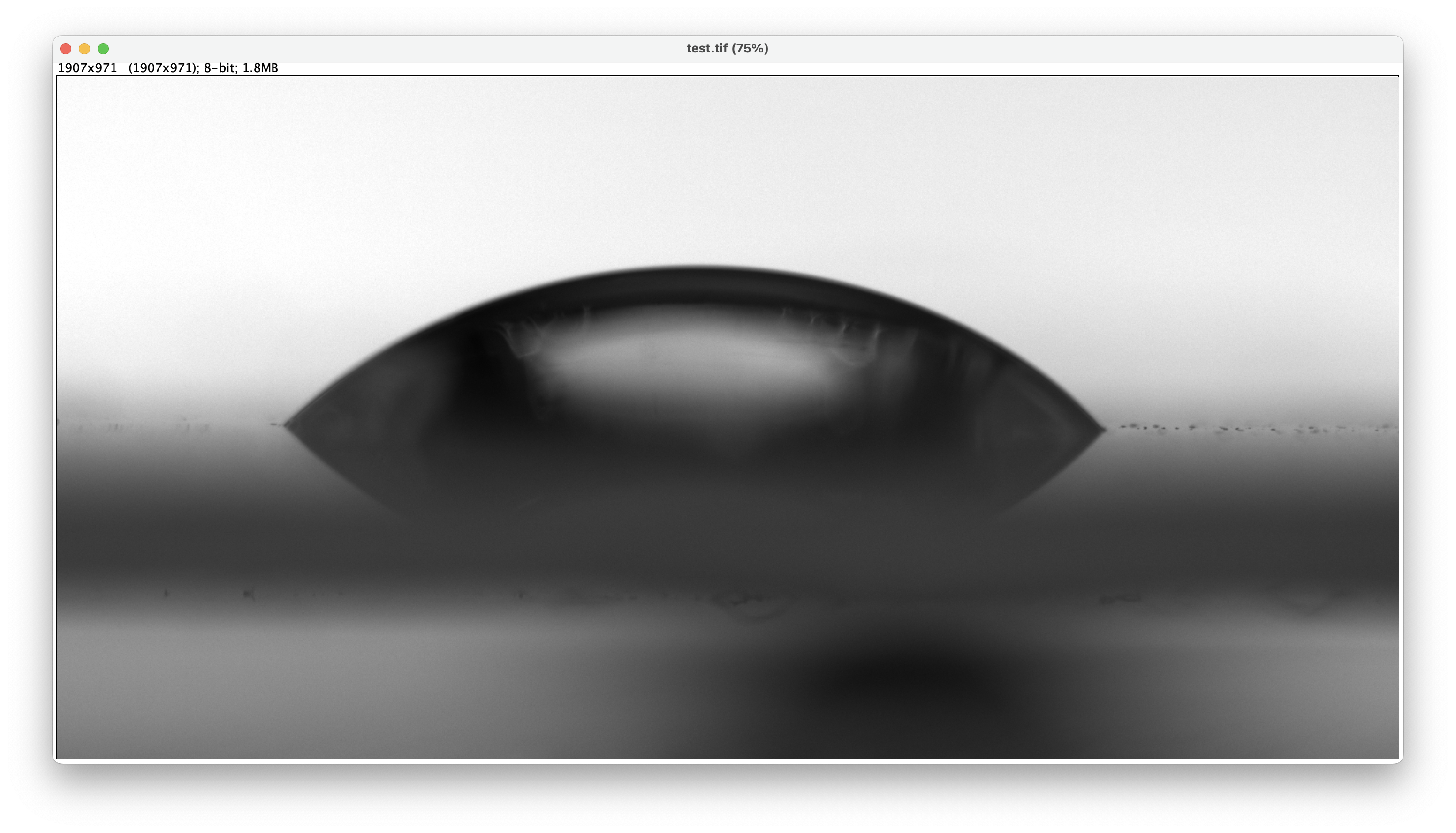
4.4 Snap an Image

Click the green Snap button.

The backend captures a full-resolution frame from the HIK camera.
If a crop ROI is active, only the cropped region is returned.
The snapped image appears in the lower card.
The raw image is also saved as a TIFF on the Raspberry Pi (/tmp/goniometer_*.tiff by default).

4.5 Automatic Measurement

After snapping, switch to the Auto tab (right panel) and click Measure (Auto).

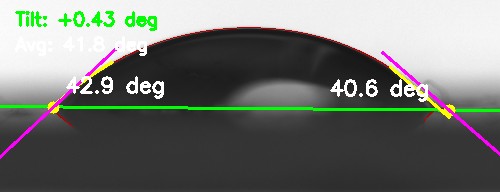
The algorithm runs in ~100 ms and overlays:

Green line — detected substrate baseline.
Cyan circles — left and right contact points.
Cyan curves — polynomial fit along each drop edge.
Magenta lines — tangent vectors at the contact points.
Angle labels — left angle θ_L and right angle θ_R in degrees.
Top-left overlay — mean angle and wetting regime (hydrophilic θ < 90° or hydrophobic θ > 90°).

The results (θ_L, θ_R, baseline tilt, regime) appear in the panel on the right.

4.6 Manual Measurement

For difficult cases (very small drops, contaminated substrates) use the Manual tab.

You place 3 points on the snapped image:

Point	How to place	Purpose
Baseline 1	Click on the substrate, left of drop	Defines substrate line
Baseline 2	Click on the substrate, right of drop	Defines substrate line
Tangent	Click on the drop edge at the contact point	Direction of drop wall

Step-by-step:

Switch to the Manual tab.
Click Place Points to enter placement mode (cursor → crosshair).
Click three times in the order above. Small numbered markers appear on the image.
Click Measure (Manual). The angle is computed from the angle between the baseline vector and the tangent vector. The result is shown immediately.

Tip: Zoom in (use the +/− buttons or scroll) and pan (click-drag) before placing points for higher accuracy.

4.7 Focus Monitor

Enable the Focus Monitor toggle in the right panel. Every 500 ms the backend computes the Laplacian variance (sharpness) of the live image and sends it back.

A progress bar shows the value relative to the session maximum. Maximize it while turning the focus ring (or the z-stage) to get the sharpest possible image before snapping.

4.8 Algorithm Configuration

Expand the Config section in the right panel to tune the image-processing parameters. You probably don't need to touch them anyway.

Parameter	Default	Effect
Canny Low	30	Lower Canny hysteresis threshold — increase for noisy images
Canny High	100	Upper Canny threshold — decrease to detect weaker edges
Blur Kernel Size	5	Gaussian pre-blur (odd numbers only) — reduce for sharp images
Local Fit Fraction	0.15	Fraction of drop width used for the tangent polynomial fit
Polynomial Degree	2	Degree of the tangent polynomial (2 = parabola, higher = more flexible)
Tangent Delta (px)	1	Finite-difference step for tangent evaluation
Angle Min (°)	1	Measurements below this are discarded as noise
Angle Max (°)	179	Measurements above this are discarded as noise

Click Reset Config to return all values to defaults. Changes are sent to the backend immediately and applied on the next measurement.

4.9 Measurement History & Export

Every successful measurement can be added to the session history:

After a successful auto or manual measurement click Add to History.
The history table shows: ID, time, mode, θ_L, θ_R.
The panel also shows a running mean ± std across all recorded values.
Use Export CSV or Export JSON to download the full table.
Click the download icon (↓) in the image card to save the annotated result image as a PNG.

5. Measurement Algorithm Explained

The algorithm is fully automatic and adapts to the wetting regime.

5.1 Preprocessing

The snapped frame is down-scaled so its longest edge ≤ 800 px (speeds up processing without losing accuracy at typical droplet sizes).
A Gaussian blur (kernel = blur_ksize) suppresses pixel noise.

5.2 Edge Detection & Contour Extraction

Canny edge detection produces a binary edge map. The largest contour (by bounding-box width) is assumed to be the drop silhouette including its mirror reflection in the substrate.

5.3 Wetting Regime Detection

The contour is profiled row by row to get width vs. vertical position. The profile is smoothed and the maximum-width row (equator) is found.

Hydrophilic (θ < 90°): No waist below the equator. The two widest points are the contact points; a tilted baseline is fitted through them.
Hydrophobic (θ > 90°): A width minimum (waist) exists below the equator — the drop overhangs the contact line. The waist row defines the baseline.

  Hydrophilic              Hydrophobic
      ___                   _____
    /     \               /       \
   |       |          ___/         \___  ← equator (widest)
    \     /               ↑
  ───┴───┴───         ────┼────────      ← waist → baseline
   contact pts         contact pts

5.4 Polynomial Tangent Fit

For each contact point a short section of the drop edge (length = fit_frac × drop_width) is fitted with a polynomial of degree poly_degree. The tangent vector is evaluated by finite differences.

Hydrophilic: polynomial y(x) — fit in the horizontal direction.
Hydrophobic: polynomial x(y) — fit in the vertical direction (avoids near-vertical tangent issues).

The contact angle θ is the angle between the tangent vector and the baseline.

6. Step-by-Step Workflow

Power on Pi + camera + LED array
Open ImSwitch in browser
Navigate to Goniometer
Set Exposure & Gain → bright, sharp live image
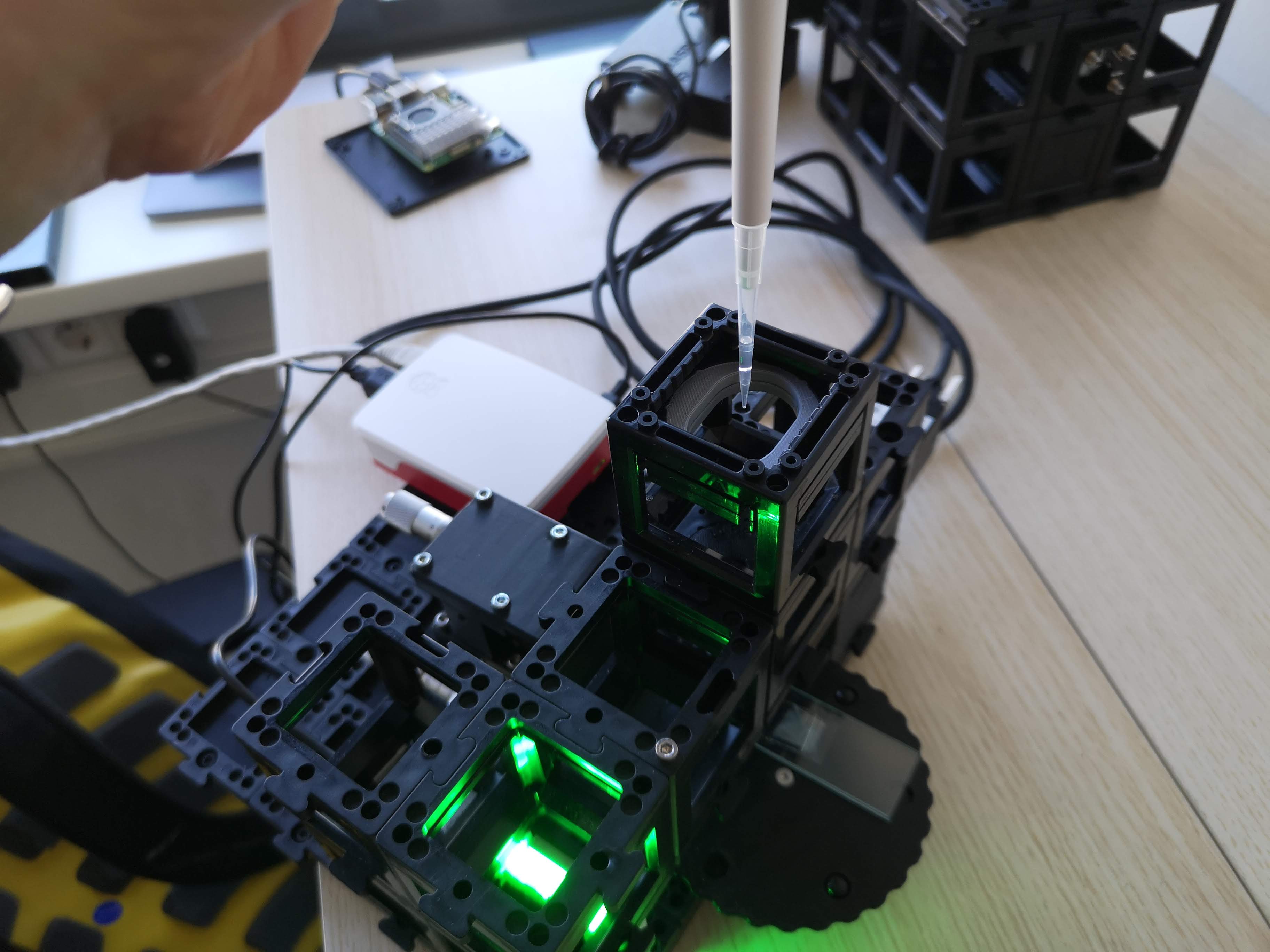
Place substrate on base plate
Dispense droplet with pipette
Check live view — is the full drop visible?
  ├── Yes → proceed to step 9
  └── No  → adjust pipette height / substrate position
(Optional) Set Crop ROI around the drop
Focus Monitor ON → maximize sharpness
Click "Snap"
Inspect snapped image
 ├── Drop clearly visible → Auto Measure
 └── Poor contrast / noise → adjust Canny / blur, re-snap
Review annotated result
 ├── Correct baseline & tangents → Add to History
 └── Wrong detection → Manual Measure or retune Config
Repeat steps 6–15 for each measurement
Export CSV / JSON when done

7. Tips for Good Results

Back-lighting should be uniform. The LED array + diffuser should produce a uniform bright background so the drop appears as a solid dark silhouette. Avoid reflections on the substrate surface.
Keep the baseline horizontal. If the substrate is tilted, the algorithm compensates (reports baseline_tilt_deg) but accuracy decreases for large tilts. Use the cube levelling feet.
Crop tightly but not too tight. Leave ~20 px of background above the top of the drop and below the substrate. The mirror reflection (below the substrate) is NOT needed — only the real drop is used.
Bring sample to focus. Use the micrometer stage to place the droplet in the image plane

Repeat and average. Dispense 5–10 drops and record each one. The mean ± std shown in the history panel is your reported contact angle.

8. Troubleshooting

Symptom	Likely cause	Fix
No live stream	Camera not detected by ImSwitch	Check USB3 cable; verify camera name in device config
"Detection failed" overlay	No contour found	Increase contrast (exposure, gain); check Canny thresholds
Wildly wrong angles	Wrong contour selected (pipette, edge)	Set crop ROI to isolate only the drop
Only one angle returned	Drop touches image border	Widen crop ROI or move drop into view
Hydrophobic/hydrophilic wrong	Waist threshold too sensitive	Increase `waist_rise_thresh` in DEFAULT_CONFIG (backend)
Baseline very tilted	Substrate not level	Level substrate; or use manual mode with explicit baseline
Focus bar stuck at low value	Wrong camera name	Verify detector name in ImSwitch config matches `GoniometerController` detector key
Export produces empty file	No measurements added to history	Click "Add to History" after each successful measurement

1. Hardware Overview​

2. Software Stack​

3. In Action​

4. UI Walkthrough​

4.1 Live Camera Stream​

4.2 Setting a Crop ROI​

4.3 Camera Settings​

4.4 Snap an Image​

4.5 Automatic Measurement​

4.6 Manual Measurement​

4.7 Focus Monitor​

4.8 Algorithm Configuration​

4.9 Measurement History & Export​

5. Measurement Algorithm Explained​

5.1 Preprocessing​

5.2 Edge Detection & Contour Extraction​

5.3 Wetting Regime Detection​

5.4 Polynomial Tangent Fit​

6. Step-by-Step Workflow​

7. Tips for Good Results​

8. Troubleshooting​